Capacitance

Related subjects: Electricity and Electronics

Background to the schools Wikipedia

SOS Children produced this website for schools as well as this video website about Africa. Before you decide about sponsoring a child, why not learn about different sponsorship charities first?

Electromagnetism

Electricity Magnetism
Electrostatics Electric charge Static electricity Electric field Conductor Insulator Triboelectricity Electrostatic discharge Induction Coulomb's law Gauss's law Electric flux / potential energy Electric dipole moment Polarization density
Magnetostatics Ampère's law Magnetic field Magnetization Magnetic flux Biot–Savart law Magnetic dipole moment Gauss's law for magnetism
Electrodynamics Lorentz force law Electromagnetic induction Faraday's law Lenz's law Displacement current Maxwell's equations Electromagnetic field Electromagnetic radiation Maxwell tensor Poynting vector Liénard–Wiechert potential Jefimenko's equations Eddy current
Electrical network Electric current Electric potential Voltage Resistance Ohm's law Series circuit Parallel circuit Direct current Alternating current Electromotive force Capacitance Inductance Impedance Resonant cavities Waveguides
Covariant formulation Electromagnetic tensor ( stress–energy tensor) Four-current Electromagnetic four-potential
Scientists Ampère Coulomb Faraday Gauss Heaviside Henry Hertz Lorentz Maxwell Tesla Volta Weber Ørsted

In electromagnetism and electronics, capacitance is the ability of a body to hold an electrical charge. Capacitance is also a measure of the amount of electrical energy stored (or separated) for a given electric potential. A common form of energy storage device is a parallel-plate capacitor. In a parallel plate capacitor, capacitance is directly proportional to the surface area of the conductor plates and inversely proportional to the separation distance between the plates. If the charges on the plates are +Q and −Q, and V gives the voltage between the plates, then the capacitance is given by

$C = \frac{Q}{V} \, .$

The SI unit of capacitance is the farad; 1 farad is 1 coulomb per volt.

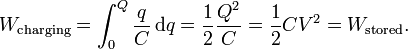
The energy (measured in joules) stored in a capacitor is equal to the work done to charge it. Consider a capacitance C, holding a charge +q on one plate and −q on the other. Moving a small element of charge dq from one plate to the other against the potential difference V = q/C requires the work dW:

$\mathrm{d}W = \frac{q}{C}\,\mathrm{d}q$

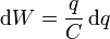
where W is the work measured in joules, q is the charge measured in coulombs and C is the capacitance, measured in farads.

The energy stored in a capacitance is found by integrating this equation. Starting with an uncharged capacitance (q = 0) and moving charge from one plate to the other until the plates have charge +Q and −Q requires the work W:

$W_\text{charging} = \int_{0}^{Q} \frac{q}{C} \, \mathrm{d}q = \frac{1}{2}\frac{Q^2}{C} = \frac{1}{2}CV^2 = W_\text{stored}.$

Capacitors

The capacitance of the majority of capacitors used in electronic circuits is several orders of magnitude smaller than the farad. The most common subunits of capacitance in use today are the millifarad (mF), microfarad (µF), nanofarad (nF) and picofarad (pF).

The capacitance can be calculated if the geometry of the conductors and the dielectric properties of the insulator between the conductors are known. For example, the capacitance of a parallel-plate capacitor constructed of two parallel plates both of area A separated by a distance d is approximately equal to the following:

$C = \varepsilon_{r}\varepsilon_{0} \frac{A}{d} \, ,$

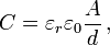
where

C is the capacitance;

A is the area of overlap of the two plates;

ε_r is the relative static permittivity (sometimes called the dielectric constant) of the material between the plates (for a vacuum, ε_r = 1);

ε₀ is the electric constant (ε₀ ≈ 8.854×10⁻¹² F m^–1); and

d is the separation between the plates.

Capacitance is proportional to the area of overlap and inversely proportional to the separation between conducting sheets. The closer the sheets are to each other, the greater the capacitance. The equation is a good approximation if d is small compared to the other dimensions of the plates so the field in the capacitor over most of its area is uniform, and the so-called fringing field around the periphery provides a small contribution. In CGS units the equation has the form:

$C = \varepsilon_{r} \frac{A}{4\pi d}$

where C in this case has the units of length.

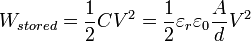
Combining the SI equation for capacitance with the above equation for the energy stored in a capacitance, for a flat-plate capacitor the energy stored is:

$W_{stored} = \frac{1}{2} C V^2 = \frac{1}{2} \varepsilon_{r}\varepsilon_{0} \frac{A}{d} V^2$ .

where W is the energy, in joules; C is the capacitance, in farads; and V is the voltage, in volts.

Voltage dependent capacitors

The dielectric constant for a number of very useful dielectrics changes as a function of the applied electrical field, for example ferroelectric materials, so the capacitance for these devices is more complex. For example, in charging such a capacitor the differential increase in voltage with charge is governed by:

$dQ = C(V) \; dV \, ,$

where the voltage dependence of capacitance, C(V), stems from the field, which in a large area parallel plate device is given by ε = V/d. This field polarizes the dielectric, which polarization, in the case of a ferroelectric, is a nonlinear S-shaped function of field, which, in the case of a large area parallel plate device, translates into a capacitance that is a nonlinear function of the voltage causing the field.

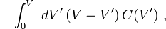
Corresponding to the voltage-dependent capacitance, to charge the capacitor to voltage V an integral relation is found:

$Q =\int_0^VdV\ C(V) \ ,$

which agrees with Q = CV only when C is voltage independent.

By the same token, the energy stored in the capacitor now is given by

$dW =Q dV =\left[ \int_0^V\ dV' \ C(V') \right] \ dV \ .$

Integrating:

$W = \int_0^V\ dV\ \int_0^V \ dV' \ C(V')$ $= \int_0^V \ dV' \ \int_{V'}^V \ dV \ C(V')$ $= \int_0^V\ dV' \left(V-V'\right) C(V') \ ,$

where interchange of the order of integration is used.

The nonlinear capacitance of a microscope probe scanned along a ferroelectric surface is used to study the domain structure of ferroelectric materials.

Another example of voltage dependent capacitance occurs in semiconductor devices such as semiconductor diodes, where the voltage dependence stems not from a change in dielectric constant but in a voltage dependence of the spacing between the charges on the two sides of the capacitor.

Frequency dependent capacitors

If a capacitor is driven with a time-varying voltage that changes rapidly enough, then the polarization of the dielectric cannot follow the signal. As an example of the origin of this mechanism, the internal microscopic dipoles contributing to the dielectric constant cannot move instantly, and so as frequency of an applied alternating voltage increases, the dipole response is limited and the dielectric constant diminishes. A changing dielectric constant with frequency is referred to as dielectric dispersion, and is governed by dielectric relaxation processes, such as Debye relaxation. Under transient conditions, the displacement field can be expressed as (see electric susceptibility):

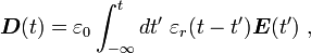
$\boldsymbol D (t) = \varepsilon_0 \int_{-\infty}^t dt' \ \varepsilon_r (t-t') \boldsymbol E (t')\ ,$

indicating the lag in response by the time dependence of ε_r, calculated in principle from an underlying microscopic analysis, for example, of the dipole behaviour in the dielectric. See, for example, linear response function. The integral extends over the entire past history up to the present time. A Fourier transform in time then results in:

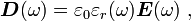
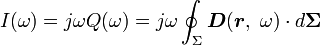
$\boldsymbol D(\omega) = \varepsilon_0 \varepsilon_r(\omega)\boldsymbol E (\omega)\ ,$

where ε_r(ω) is now a complex function, with an imaginary part related to absorption of energy from the field by the medium. See permittivity. The capacitance, being proportional to the dielectric constant, also exhibits this frequency behaviour. Fourier transforming Gauss's law with this form for displacement field:

$I(\omega) = j\omega Q(\omega) = j\omega \oint_{\Sigma} \boldsymbol D (\boldsymbol r , \ \omega)\cdot d \boldsymbol{\Sigma} \$

$=\left[ G(\omega) + j \omega C(\omega)\right] V(\omega) = \frac {V(\omega)}{Z(\omega)} \ ,$

where j is the imaginary unit, V(ω) is the voltage component at angular frequency ω, G(ω) is the real part of the current, called the conductance, and C(ω) determines the imaginary part of the current and is the capacitance. Z(ω) is the complex impedance.

When a parallel-plate capacitor is filled with a dielectric, the measurement of dielectric properties of the medium is based upon the relation:

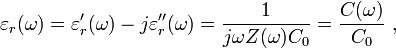
$\varepsilon_r(\omega) = \varepsilon '_r(\omega) - j \varepsilon ''_r(\omega) = \frac{1}{j\omega Z(\omega) C_0} = \frac{C(\omega)}{C_0} \ ,$

where a single prime denotes the real part and a double prime the imaginary part, Z(ω) is the complex impedance with the dielectric present, C(ω) is the so-called complex capacitance with the dielectric present, and C₀ is the capacitance without the dielectric. (Measurement "without the dielectric" in principle means measurement in free space, an unattainable goal inasmuch as even the quantum vacuum is predicted to exhibit nonideal behaviour, such as dichroism. For practical purposes, when measurement errors are taken into account, often a measurement in terrestrial vacuum, or simply a calculation of C₀, is sufficiently accurate. )

Using this measurement method, the dielectric constant may exhibit a resonance at certain frequencies corresponding to characteristic response frequencies (excitation energies) of contributors to the dielectric constant. These resonances are the basis for a number of experimental techniques for detecting defects. The conductance method measures absorption as a function of frequency. Alternatively, the time response of the capacitance can be used directly, as in deep-level transient spectroscopy.

Another example of frequency dependent capacitance occurs with MOS capacitors, where the slow generation of minority carriers means that at high frequencies the capacitance measures only the majority carrier response, while at low frequencies both types of carrier respond.

At optical frequencies, in semiconductors the dielectric constant exhibits structure related to the band structure of the solid. Sophisticated modulation spectroscopy measurement methods based upon modulating the crystal structure by pressure or by other stresses and observing the related changes in absorption or reflection of light have advanced our knowledge of these materials.

Capacitance matrix

The discussion above is limited to the case of two conducting plates, although of arbitrary size and shape. The definition C=Q/V still holds for a single plate given a charge, in which case the field lines produced by that charge terminate as if the plate were at the centre of an oppositely charged sphere at infinity.

$C = Q/V$ does not apply when there are more than two charged plates, or when the net charge on the two plates is non-zero. To handle this case, Maxwell introduced his "coefficients of potential". If three plates are given charges $Q_1, Q_2, Q_3$ , then the voltage of plate 1 is given by

$V_1 = P_{11}Q_1 + P_{12} Q_2 + P_{13}Q_3$ ,

and similarly for the other voltages. Maxwell showed that the coefficients of potential are symmetric, so that $P_{12}=P_{21}$ , etc. Thus the system can be described by a collection of coefficients known as the "Reciprocal Capacitance Matrix"is used, which is defined as:

$P_{ij} = \frac{V_{i}}{Q_{j}}$

From this, the mutual capacitance $C_{m}$ between two objects can be defined by solving for the total charge Q and using $C_{m}=Q/V$ .

$C_{m} = \frac{V}{(P_{11} + P_{22})-(P_{12} + P_{21})}$

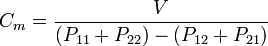
Since no actual device holds perfectly equal and opposite charges on each of the two "plates", it is the mutual capacitance that is reported on capacitors. The collection of coefficients $C_{ij} = Q_{i}/V_{j}$ is known as the capacitance matrix and also describes the capacitance of the system.

Self-capacitance

In electrical circuits, the term capacitance is usually a shorthand for the mutual capacitance between two adjacent conductors, such as the two plates of a capacitor. There also exists a property called self-capacitance, which is the amount of electrical charge that must be added to an isolated conductor to raise its electrical potential by one volt. The reference point for this potential is a theoretical hollow conducting sphere, of infinite radius, centered on the conductor. Using this method, the self-capacitance of a conducting sphere of radius R is given by:

$C=4\pi\varepsilon_0R \,$

Example values of self-capacitance are:

for the top "plate" of a van de Graaff generator, typically a sphere 20 cm in radius: 20 pF
the planet Earth: about 700 nF

Elastance

The inverse of capacitance is called elastance. The unit of elastance is the daraf.

Stray capacitance

Any two adjacent conductors can be considered a capacitor, although the capacitance will be small unless the conductors are close together for long. This (often unwanted) effect is termed "stray capacitance". Stray capacitance can allow signals to leak between otherwise isolated circuits (an effect called crosstalk), and it can be a limiting factor for proper functioning of circuits at high frequency.

Stray capacitance is often encountered in amplifier circuits in the form of "feedthrough" capacitance that interconnects the input and output nodes (both defined relative to a common ground). It is often convenient for analytical purposes to replace this capacitance with a combination of one input-to-ground capacitance and one output-to-ground capacitance. (The original configuration — including the input-to-output capacitance — is often referred to as a pi-configuration.) Miller's theorem can be used to effect this replacement. Miller's theorem states that, if the gain ratio of two nodes is 1/K, then an impedance of Z connecting the two nodes can be replaced with a Z/(1-k) impedance between the first node and ground and a KZ/(K-1) impedance between the second node and ground. (Since impedance varies inversely with capacitance, the internode capacitance, C, will be seen to have been replaced by a capacitance of KC from input to ground and a capacitance of (K-1)C/K from output to ground.) When the input-to-output gain is very large, the equivalent input-to-ground impedance is very small while the output-to-ground impedance is essentially equal to the original (input-to-output) impedance.

Capacitance of simple systems

Calculating the capacitance of a system amounts to solving the Laplace equation ∇²φ=0 with a constant potential φ on the surface of the conductors. This is trivial in cases with high symmetry. There is no solution in terms of elementary functions in more complicated cases.

For quasi two-dimensional situations analytic functions may be used to map different geometries to each other. See also Schwarz-Christoffel mapping.

Capacitance of simple systems
Type	Capacitance	Comment
Parallel-plate capacitor	$\varepsilon A /d$	A: Area d: Distance ε: Permittivity
Coaxial cable	$\frac{2\pi \varepsilon l}{\ln \left( a_{2}/a_{1}\right) }$	a₁: Inner radius a₂: Outer radius $l$ : Length
Pair of parallel wires	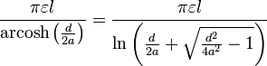$\frac{\pi \varepsilon l}{\operatorname{arcosh}\left( \frac{d}{2a}\right) }=\frac{\pi \varepsilon l}{\ln \left( \frac{d}{2a}+\sqrt{\frac{d^{2}}{4a^{2}}-1}\right) }$	a: Wire radius d: Distance, d > 2a $l$ : Length of pair
Wire parallel to wall	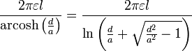$\frac{2\pi \varepsilon l}{\operatorname{arcosh}\left( \frac{d}{a}\right) }=\frac{2\pi \varepsilon l}{\ln \left( \frac{d}{a}+\sqrt{\frac{d^{2}}{a^{2}}-1}\right) }$	a: Wire radius d: Distance, d > a $l$ : Wire length
Two parallel coplanar strips	$\varepsilon l \frac{ K\left( \sqrt{1-k^{2}} \right) }{ K\left(k \right) }$	d: Distance w₁, w₂: Strip width k_i: d/(2w_i+d) k²: k₁k₂ K: Elliptic integral $l$ : Length
Concentric spheres	$\frac{4\pi \varepsilon a_{1}a_{2}}{a_{2}-a_{1}}$	a₁: Inner radius a₂: Outer radius
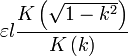
Two spheres, equal radius	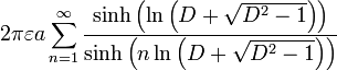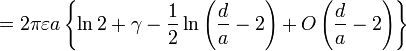$2\pi \varepsilon a\sum_{n=1}^{\infty }\frac{\sinh \left( \ln \left( D+\sqrt{D^{2}-1}\right) \right) }{\sinh \left( n\ln \left( D+\sqrt{ D^{2}-1}\right) \right) }$ $=2\pi \varepsilon a\left\{ 1+\frac{1}{2D}+\frac{1}{4D^{2}}+\frac{1}{8D^{3}}+\frac{1}{8D^{4}}+\frac{3}{32D^{5}}+O\left( \frac{1}{D^{6}}\right) \right\}$ $=2\pi \varepsilon a\left\{ \ln 2+\gamma -\frac{1}{2}\ln \left( \frac{d}{a}-2\right) +O\left( \frac{d}{a}-2\right) \right\}$	a: Radius d: Distance, d > 2a D = d/2a γ: Euler's constant
Sphere in front of wall	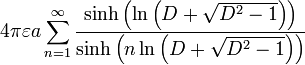$4\pi \varepsilon a\sum_{n=1}^{\infty }\frac{\sinh \left( \ln \left( D+\sqrt{D^{2}-1}\right) \right) }{\sinh \left( n\ln \left( D+\sqrt{ D^{2}-1}\right) \right) }$	a: Radius d: Distance, d > a D = d/a
Sphere	$4\pi \varepsilon a$	a: Radius
Circular disc	$8\varepsilon a$	a: Radius
Thin straight wire, finite length	$\frac{2\pi \varepsilon l}{\Lambda }\left\{ 1+\frac{1}{\Lambda }\left( 1-\ln 2\right) +\frac{1}{\Lambda ^{2}}\left[ 1+\left( 1-\ln 2\right) ^{2}-\frac{\pi ^{2}}{12}\right] +O\left(\frac{1}{\Lambda ^{3}}\right) \right\}$	a: Wire radius $l$ : Length Λ: ln( $l$ /a)

Retrieved from " http://en.wikipedia.org/w/index.php?title=Capacitance&oldid=403536009"