Chapter 20 Money Demand

Chapter Objectives

By the end of this chapter, students should be able to:

Describe Friedman’s modern quantity theory of money.
Describe the classical quantity theory.
Describe Keynes’s liquidity preference theory and its improvements.
Contrast the modern quantity theory with the liquidity preference theory.

20.1 The Quantity Theory

Learning Objective

What is the quantity theory of money and how was it improved by Milton Friedman?

The rest of this book is about monetary theory, a daunting-sounding term. It’s not the easiest aspect of money and banking, but it isn’t terribly taxing either so there is no need to freak out. We’re going to take it nice and slow. And here’s a big hint: you already know most of the outcomes because we’ve discussed them already in more intuitive terms. In the chapters that follow, we’re simply going to provide you with more formal ways of thinking about how the money supply determines output (Y*) and the price level (P*).

We’ve already discussed the money supply at some length in the chapters above, so we’ll start our theorizing with the demand for money, specifically John Maynard Keynes’s liquidity preference theory and Milton Friedman’s modern quantity theory of money. Building on the work of earlier scholars, including Irving Fisher of Fisher Equation fame, the late, great Friedman treats money like any other asset, concluding that economic agents (individuals, firms, governments) want to hold a certain quantity of real, as opposed to nominal, money balances. If inflation erodes the purchasing power of the unit of account, economic agents will want to hold higher nominal balances to compensate, to keep their real money balances constant. The level of those real balances, Friedman argued, was a function of permanent income (the present discounted value of all expected future income), the relative expected return on bonds and stocks versus money, and expected inflation.

More formally,

M_{d} / P : f (Y p <+>, r_{b} - r_{m} <->, r_{s} - r_{m} <->, π^{e} - r_{m} <->)

where:

M_d/P = demand for real money balances (M_d = money demand; P = price level)

f means “function of” (not equal to)

Y_p = permanent income

r_b – r_m = the expected return on bonds minus the expected return on money

r_s – r_m = the expected return on stocks (equities) minus the expected return on money

π^e – r_m = expected inflation minus the expected return on money

<+> = varies directly with

<−> = varies indirectly with

So the demand for real money balances, according to Friedman, increases when permanent income increases and declines when the expected returns on bonds, stocks, or goods increases versus the expected returns on money, which includes both the interest paid on deposits and the services banks provide to depositors.

Stop and Think Box

As noted in the text, money demand is where the action is these days because, as we learned in previous chapters, the central bank determines what the money supply will be, so we can model it as a vertical line. Earlier monetary theorists, however, had no such luxury because, under a specie standard, money was supplied exogenously. What did the supply curve look like before the rise of modern central banking in the twentieth century?

The supply curve sloped upward, as most do. You can think of this in two ways, first, by thinking of interest on the vertical axis. Interest is literally the price of money. When interest is high, more people want to supply money to the system because seigniorage is higher. So more people want to form banks or find other ways of issuing money, extant bankers want to issue more money (notes and/or deposits), and so forth. You can also think of this in terms of the price of gold. When its price is low, there is not much incentive to go out and find more of it because you can earn just as much making cheesecake or whatever. When the price of gold is high, however, everybody wants to go out and prospect for new veins or for new ways of extracting gold atoms from what looks like plain old dirt. The point is that early monetary theorists did not have the luxury of concentrating on the nature of money demand; they also had to worry about the nature of money supply.

This all makes perfectly good sense when you think about it. If people suspect they are permanently more wealthy, they are going to want to hold more money, in real terms, so they can buy caviar and fancy golf clubs and what not. If the return on financial investments decreases vis-à-vis money, they will want to hold more money because its opportunity cost is lower. If inflation expectations increase, but the return on money doesn’t, people will want to hold less money, ceteris paribus, because the relative return on goods (land, gold, turnips) will increase. (In other words, expected inflation here proxies the expected return on nonfinancial goods.)

Key Takeaways

According to Milton Friedman, demand for real money balances (M_d/P) is directly related to permanent income (Y_p)—the discounted present value of expected future income—and indirectly related to the expected differential returns from bonds, stocks (equities), and goods vis-à-vis money (r_b – r_m, r_s – r_m, π^e – r_m ), where inflation (π) proxies the return on goods.
Because he believed that the return on money would increase (decrease) as returns on bonds, stocks, and goods increased (decreased), Friedman did not think that interest rate changes mattered much.

20.2 Liquidity Preference Theory

Learning Objective

What is the liquidity preference theory and how has it been improved?

The very late and very great John Maynard Keynes (to distinguish him from his father, economist John Neville Keynes) developed the liquidity preference theory in response to the rather primitive pre-Friedman quantity theory of money, which was simply an assumption-laden identity called the equation of exchange:

M V = P Y

where:

M = money supply

V = velocity

P = price level

Y = output

Nobody doubted the equation itself, which, as an identity (like x = x), is undeniable. But many doubted the way that classical quantity theorists used the equation of exchange as the causal statement: increases in the money supply lead to proportional increases in the price level. The classical quantity theory also suffered by assuming that money velocity, the number of times per year a unit of currency was spent, was constant. Although a good first approximation of reality, the classical quantity theory, which critics derided as the “naïve quantity theory of money,” was hardly the entire story. In particular, it could not explain why velocity was pro-cyclical, i.e., why it increased during business expansions and decreased during recessions.

To find a better theory, Keynes took a different point of departure, asking in effect, “Why do economic agents hold money?” He came up with three reasons:

Transactions: Economic agents need money to make payments. As their incomes rise, so, too, do the number and value of those payments, so this part of money demand is proportional to income.
Precautions: S—t happens was a catch phrase of the 1980s, recalled perhaps most famously in the hit movie Forrest Gump. Way back in the 1930s, Keynes already knew that bad stuff happens—and that one defense against it was to keep some spare cash lying around as a precaution. It, too, is directly proportional to income, Keynes believed.
Speculations: People will hold more bonds than money when interest rates are high for two reasons. The opportunity cost of holding money (which Keynes assumed has zero return) is higher and the expectation is that interest rates will fall, raising the price of bonds. When interest rates are low, the opportunity cost of holding money is low, and the expectation is that rates will rise, decreasing the price of bonds. So people hold larger money balances when rates are low. Overall, then, money demand and interest rates are inversely related.

More formally, Keynes’s ideas can be stated as

M_{d} / P = f (i <->, Y <+>)

where:

Md/P = demand for real money balances

f means “function of” (this simplifies the mathematics)

i = interest rate

Y = output (income)

<+> = varies directly with

<−> = varies indirectly with

An increase in interest rates induces people to decrease real money balances for a given income level, implying that velocity must be higher. So Keynes’s view was superior to the classical quantity theory of money because he showed that velocity is not constant but rather is positively related to interest rates, thereby explaining its pro-cyclical nature. (Recall from Chapter 5 "The Economics of Interest-Rate Fluctuations" that interest rates rise during expansions and fall during recessions.) Keynes’s theory was also fruitful because it induced other scholars to elaborate on it further.

In the early 1950s, for example, a young Will Baumolhttp://pages.stern.nyu.edu/~wbaumol/ and James Tobinhttp://nobelprize.org/nobel_prizes/economics/laureates/1981/tobin-autobio.html independently showed that money balances, held for transaction purposes (not just speculative ones), were sensitive to interest rates, even if the return on money was zero. That is because people can hold bonds or other interest-bearing securities until they need to make a payment. When interest rates are high, people will hold as little money for transaction purposes as possible because it will be worth the time and trouble of investing in bonds and then liquidating them when needed. When rates are low, by contrast, people will hold more money for transaction purposes because it isn’t worth the hassle and brokerage fees to play with bonds very often. So transaction demand for money is negatively related to interest rates. A similar trade-off applies also to precautionary balances. The lure of high interest rates offsets the fear of bad events occurring. When rates are low, better to play it safe and hold more dough. So the precautionary demand for money is also negatively related to interest rates.

Key Takeaways

Before Friedman, the quantity theory of money was a much simpler affair based on the so-called equation of exchange—money times velocity equals the price level times output (MV = PY)—plus the assumptions that changes in the money supply cause changes in output and prices and that velocity changes so slowly it can be safely treated as a constant. Note that the interest rate is not considered at all in this so-called naïve version.
Keynes and his followers knew that interest rates were important to money demand and that velocity wasn’t a constant, so they created a theory whereby economic actors demand money to engage in transactions (buy and sell goods), as a precaution against unexpected negative shocks, and as a speculation.
Due to the first two motivations, real money balances increase directly with output.
Due to the speculative motive, real money balances and interest rates are inversely related. When interest rates are high, so is the opportunity cost of holding money.
Throw in the expectation that rates will likely fall, causing bond prices to rise, and people are induced to hold less money and more bonds.
When interest rates are low, by contrast, people expect them to rise, which will hurt bond prices. Moreover, the opportunity cost of holding money to make transactions or as a precaution against shocks is low when interest rates are low, so people will hold more money and fewer bonds when interest rates are low.

20.3 Head to Head: Friedman versus Keynes

Learning Objective

How do the modern quantity theory and the liquidity preference theory compare?

Friedman’s elaboration of the quantity theory drew heavily on Keynes’s and his followers’ insights as well, so it is not surprising that Friedman’s view eventually predominated. The modern quantity theory is superior to Keynes’s liquidity preference theory because it is more complex, specifying three types of assets (bonds, equities, goods) instead of just one (bonds). It also does not assume that the return on money is zero, or even a constant. In Friedman’s theory, velocity is no longer a constant; instead, it is highly predictable and, as in reality and Keynes’s formulation, pro-cyclical, rising during expansions and falling during recessions.

Finally, unlike the liquidity preference theory, Friedman’s modern quantity theory predicts that interest rate changes should have little effect on money demand. The reason for this is that Friedman believed that the return on bonds, stocks, goods, and money would be positively correlated, leading to little change in r_b – r_m, r_s – r_m, or π^e – r_m because both sides would rise or fall about the same amount. That insight essentially reduces the modern quantity theory to Md/P = f(Y_p <+>). Until the 1970s, Friedman was more or less correct. Interest rates did not strongly affect the demand for money, so velocity was predictable and the quantity of money was closely linked to aggregate output. Except when nominal interest rates hit zero (as in Japan), the demand for money was somewhat sensitive to interest rates, so there was no so-called liquidity trap (where money demand is perfectly horizontal, leaving central bankers impotent). During the 1970s, however, money demand became more sensitive to interest rate changes, and velocity, output, and inflation became harder to predict. That’s one reason, noted in Chapter 17 "Monetary Policy Targets and Goals", why central banks in the 1970s found that targeting monetary aggregates did not help them to meet their inflation or output goals.

Stop and Think Box

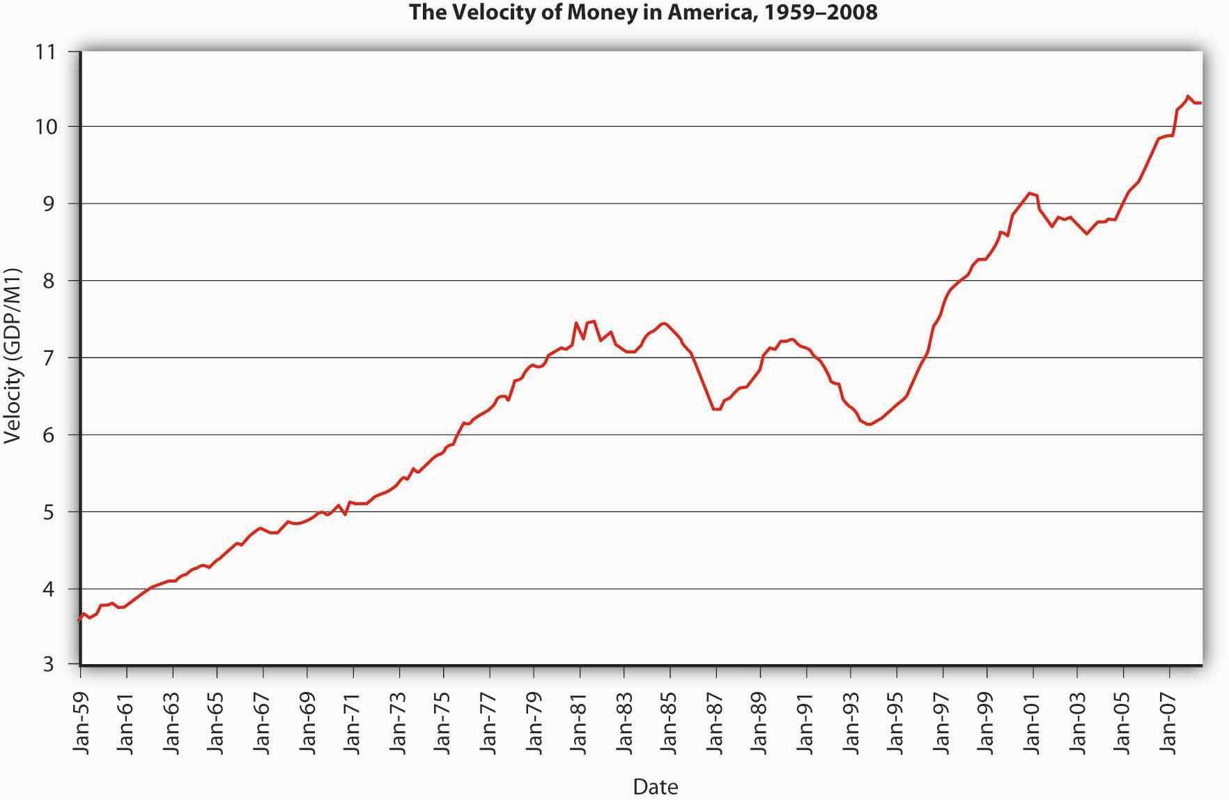
Stare at Figure 20.1 "The quarterly volatility of velocity, 1959–2008" for a spell. How is it related to the discussion in this chapter? Then take a gander at Figure 20.2 "The velocity of money in the United States, 1959–2008". In addition to giving us a new perspective on Figure 20.1 "The quarterly volatility of velocity, 1959–2008", it shows that the velocity of money (velocity = GDP/M1 because MV = PY can be solved for V: V = PY/M) has increased considerably since the late 1950s. Why might that be?

Figure 20.1 The quarterly volatility of velocity, 1959–2008

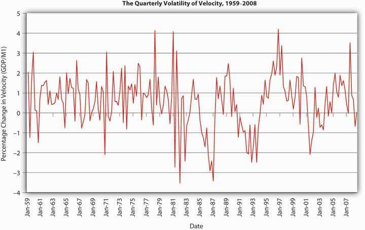
Figure 20.2 The velocity of money in the United States, 1959–2008

The chapter makes the point that velocity became much less stable and much less predictable in the 1970s and thereafter. Figure 20.1 "The quarterly volatility of velocity, 1959–2008" shows that by measuring the quarterly change in velocity. Before 1970, velocity went up and down between −1 and 3 percent in pretty regular cycles. Thereafter, the variance increased to between almost −4 and 4 percent, and the pattern has become much less regular. This is important because it shows why Friedman’s modern quantity theory of money lost much of its explanatory power in the 1970s, leading to changes in central bank targeting and monetary theory.

Figure 20.2 "The velocity of money in the United States, 1959–2008" suggests that velocity likely increased in the latter half of the twentieth century due to technological improvements that allowed each unit of currency to be used in more transactions over the course of a year. More efficient payment systems (electronic funds transfer), increased use of credit, lower transaction costs, and financial innovations like cash management accounts have all helped to increase V, to help each dollar move through more hands or the same number of hands in less time.

The breakdown of the quantity theory had severe repercussions for central banking, central bankers, and monetary theorists. That was bad news for them (and for people like Wright who grew up in that awful decade), and it is bad news for us because our exploration of monetary theory must continue. Monetary economists have learned a lot over the last few decades by constantly testing, critiquing, and improving models like those of Keynes and Friedman, and we’re going to follow along so you’ll know precisely where monetary theory and policy stand at present.

Stop and Think Box

Examine Figure 20.3 "Velocity of money, 1790–1860", Figure 20.4 "U.S. national debt, 1790–1860", and Figure 20.5 "Volume of public securities trading in select U.S. markets, by year, 1790–1834" carefully. Why might velocity have trended upward to approximately 1815 and then fallen? Hint: Alexander Hamilton argued in the early 1790s that “in countries in which the national debt is properly funded, and an object of established confidence, it answers most of the purposes of money. Transfers of stock or public debt are there equivalent to payments in specie; or in other words, stock, in the principal transactions of business, passes current as specie. The same thing would, in all probability happen here, under the like circumstances”—if his funding plan was adopted. It was.

Figure 20.3 Velocity of money, 1790–1860

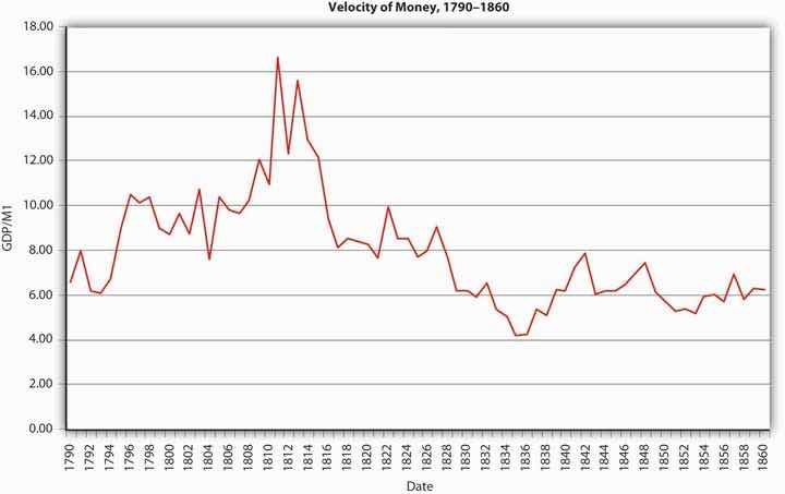
Figure 20.4 U.S. national debt, 1790–1860

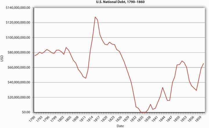
Figure 20.5 Volume of public securities trading in select U.S. markets, by year, 1790–1834

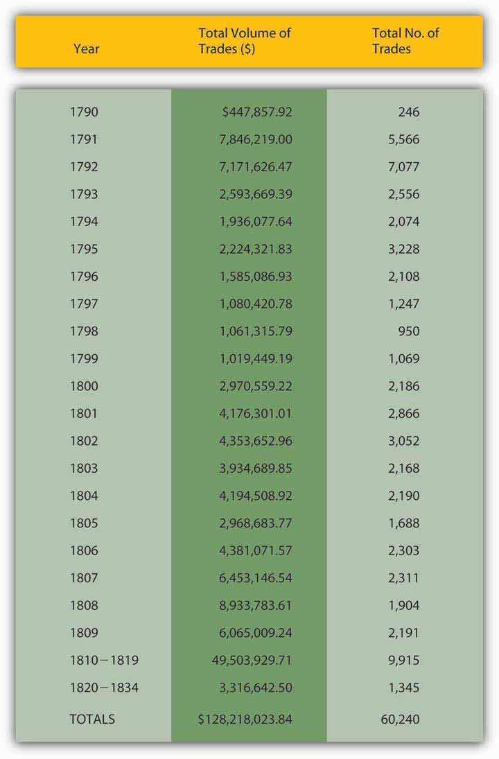
Velocity rises when there are money substitutes, highly liquid assets that allow economic agents to earn interest. Apparently Hamilton was right—the national debt answered most of the purposes of money. Ergo, not as much M1 was needed to support the gross domestic product (GDP) and price level, so velocity rose during the period that the debt was large. It then dropped as the government paid off the debt, requiring the use of more M1.

Key Takeaways

Friedman’s modern quantity theory proved itself superior to Keynes’s liquidity preference theory because it was more complex, accounting for equities and goods as well as bonds.
Friedman allowed the return on money to vary and to increase above zero, making it more realistic than Keynes’s assumption of zero return.
Money demand was indeed somewhat sensitive to interest rates but velocity, while not constant, was predictable, making the link between money and prices that Friedman predicted a close one.
Friedman’s reformulation of the quantity theory held up well only until the 1970s, when it cracked asunder because money demand became more sensitive to interest rate changes, thus causing velocity to vacillate unpredictably and breaking the close link between the quantity of money and output and inflation.

20.4 Suggested Reading

Friedman, Milton. Money Mischief: Episodes in Monetary History. New York: Harvest, 1994.

Friedman, Milton, and Anna Jacobson. A Monetary History of the United States, 1867–1960 (Princeton, NJ: Princeton University Press, 1971).

Kindleberger, Charles. Keynesianism vs. Monetarism and Other Essays in Financial History. London: George Allen & Unwin, 1985.

Minsky, Hyman. John Maynard Keynes. New York: McGraw-Hill, 2008)

Serletis, Apostolos. The Demand for Money: Theoretical and Empirical Approaches. New York: Springer, 2007.