When to Use These Tests

In statistics, "ranking" refers to the data transformation in which numerical or ordinal values are replaced by their rank when the data are sorted. If, for example, the numerical data 3.4, 5.1, 2.6, 7.3 are observed, the ranks of these data items would be 2, 3, 1 and 4 respectively. In another example, the ordinal data hot, cold, warm would be replaced by 3, 1, 2. In these examples, the ranks are assigned to values in ascending order. (In some other cases, descending ranks are used. ) Ranks are related to the indexed list of order statistics, which consists of the original dataset rearranged into ascending order.

Some kinds of statistical tests employ calculations based on ranks. Examples include:

• Friedman test
• Kruskal-Wallis test
• Rank products
• Spearman's rank correlation coefficient
• Wilcoxon rank-sum test
• Wilcoxon signed-rank test

Some ranks can have non-integer values for tied data values. For example, when there is an even number of copies of the same data value, the above described fractional statistical rank of the tied data ends in $\frac{1}{2}$.

Data Transformation

Data transformation refers to the application of a deterministic mathematical function to each point in a data set—that is, each data point $z_i$ is replaced with the transformed value $y_i = f(z_i)$, where $f$ is a function. Transforms are usually applied so that the data appear to more closely meet the assumptions of a statistical inference procedure that is to be applied, or to improve the interpretability or appearance of graphs.

Nearly always, the function that is used to transform the data is invertible and, generally, is continuous. The transformation is usually applied to a collection of comparable measurements. For example, if we are working with data on peoples' incomes in some currency unit, it would be common to transform each person's income value by the logarithm function.

Reasons for Transforming Data

Guidance for how data should be transformed, or whether a transform should be applied at all, should come from the particular statistical analysis to be performed. For example, a simple way to construct an approximate 95% confidence interval for the population mean is to take the sample mean plus or minus two standard error units. However, the constant factor 2 used here is particular to the normal distribution and is only applicable if the sample mean varies approximately normally. The central limit theorem states that in many situations, the sample mean does vary normally if the sample size is reasonably large.

However, if the population is substantially skewed and the sample size is at most moderate, the approximation provided by the central limit theorem can be poor, and the resulting confidence interval will likely have the wrong coverage probability. Thus, when there is evidence of substantial skew in the data, it is common to transform the data to a symmetric distribution before constructing a confidence interval. If desired, the confidence interval can then be transformed back to the original scale using the inverse of the transformation that was applied to the data.

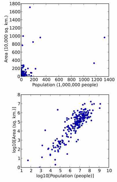
Data can also be transformed to make it easier to visualize them. For example, suppose we have a scatterplot in which the points are the countries of the world, and the data values being plotted are the land area and population of each country. If the plot is made using untransformed data (e.g., square kilometers for area and the number of people for population), most of the countries would be plotted in tight cluster of points in the lower left corner of the graph. The few countries with very large areas and/or populations would be spread thinly around most of the graph's area. Simply rescaling units (e.g., to thousand square kilometers, or to millions of people) will not change this. However, following logarithmic transformations of both area and population, the points will be spread more uniformly in the graph .

Population Versus Area Scatterplots

A scatterplot in which the areas of the sovereign states and dependent territories in the world are plotted on the vertical axis against their populations on the horizontal axis. The upper plot uses raw data. In the lower plot, both the area and population data have been transformed using the logarithm function.

A final reason that data can be transformed is to improve interpretability, even if no formal statistical analysis or visualization is to be performed. For example, suppose we are comparing cars in terms of their fuel economy. These data are usually presented as "kilometers per liter" or "miles per gallon. " However, if the goal is to assess how much additional fuel a person would use in one year when driving one car compared to another, it is more natural to work with the data transformed by the reciprocal function, yielding liters per kilometer, or gallons per mile.