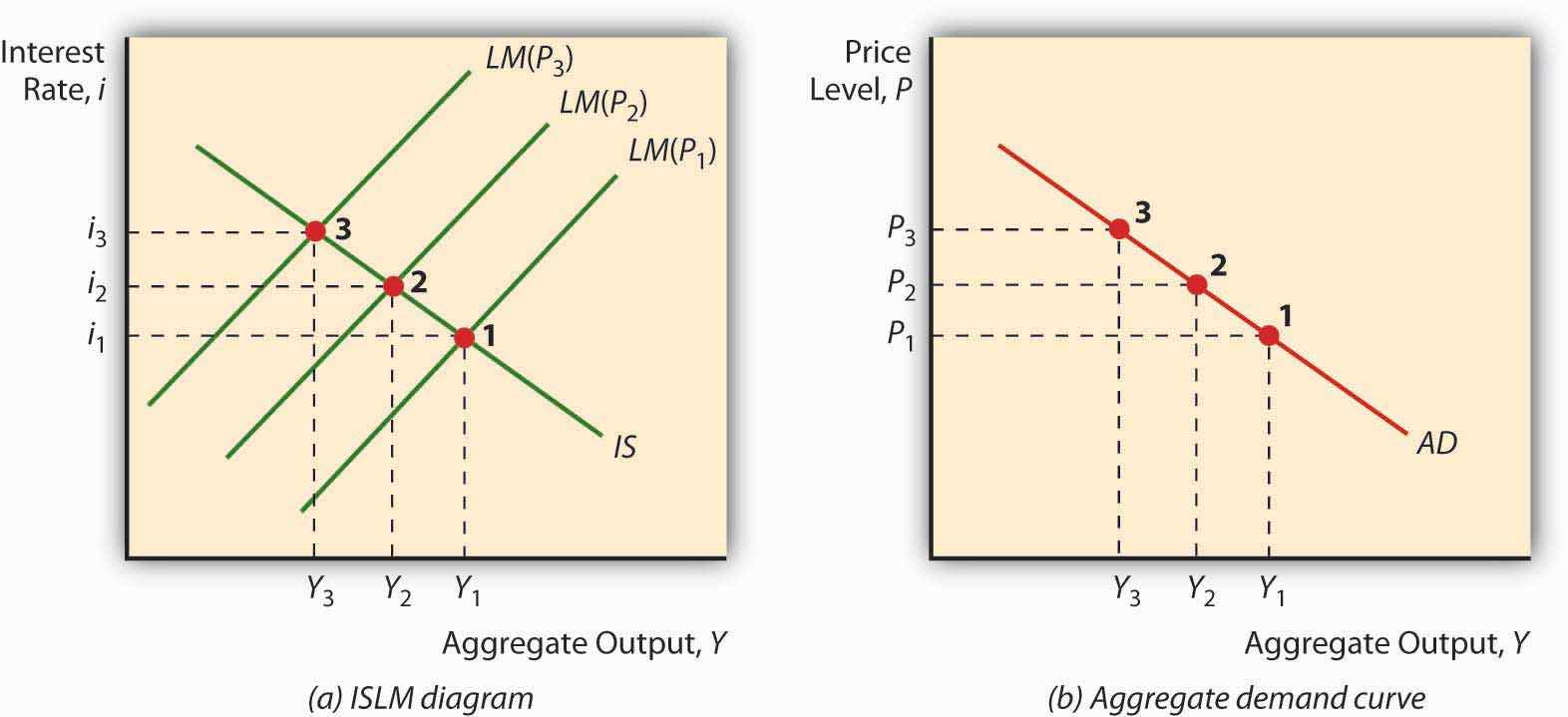
Imagine a fixed IS curve and an LM curve shifting hard left due to increases in the price level, as in Figure 22.6 "Deriving the aggregate demand curve". As prices increase, Y falls and i rises. Now plot that outcome on a new graph, where aggregate output Y remains on the horizontal axis but the vertical axis is replaced by the price level P. The resulting curve, called the aggregate demand (AD) curve, will slope downward, as below. The AD curve is a very powerful tool because it indicates the points at which equilibrium is achieved in the markets for goods and money at a given price level. It slopes downward because a high price level, ceteris paribus, means a small real money supply, high interest rates, and a low level of output, while a low price level, all else constant, is consistent with a larger real money supply, low interest rates, and kickin’ output.
Figure 22.6 Deriving the aggregate demand curve

Because the AD curve is essentially just another way of stating the IS-LM model, anything that would change the IS or LM curves will also shift the AD curve. More specifically, the AD curve shifts in the same direction as the IS curve, so it shifts right (left) with autonomous increases (decreases) in C, I, G, and NX and decreases (increases) in T. The AD curve also shifts in the same direction as the LM curve. So if MS increases (decreases), it shifts right (left), and if Md increases (decreases) it shifts left (right), as in Figure 22.3 "Predicted effects of changes in major macroeconomic variables".