Like the geoprocessing tools available for use on vector datasets (Section 8.1 "Basic Geoprocessing with Rasters"), raster data can undergo similar spatial operations. Although the actual computation of these operations is significantly different from their vector counterparts, their conceptual underpinning is similar. The geoprocessing techniques covered here include both single layer (Section 8.1.1 "Single Layer Analysis") and multiple layer (Section 8.1.2 "Multiple Layer Analysis") operations.
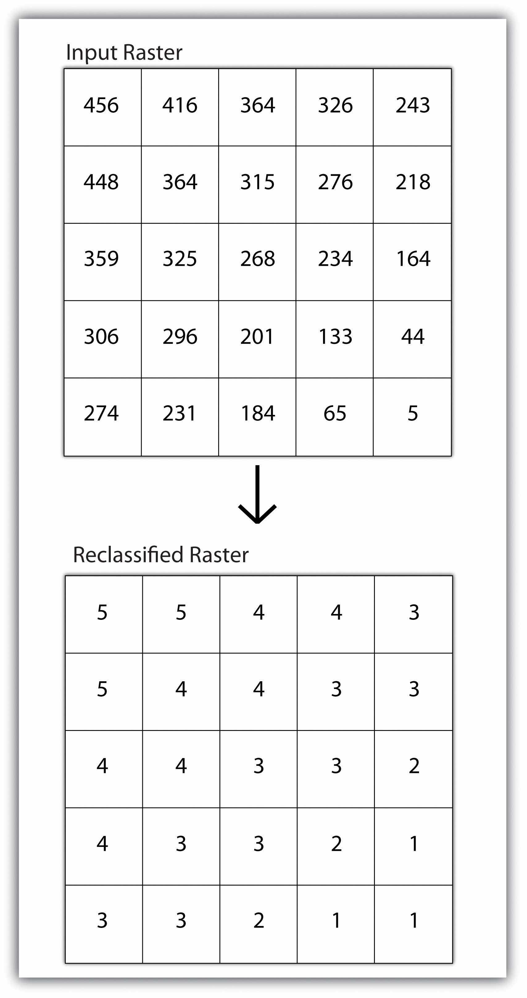
Reclassifying, or recoding, a dataset is commonly one of the first steps undertaken during raster analysis. Reclassification is basically the single layer process of assigning a new class or range value to all pixels in the dataset based on their original values (Figure 8.1 "Raster Reclassification". For example, an elevation grid commonly contains a different value for nearly every cell within its extent. These values could be simplified by aggregating each pixel value in a few discrete classes (i.e., 0–100 = “1,” 101–200 = “2,” 201–300 = “3,” etc.). This simplification allows for fewer unique values and cheaper storage requirements. In addition, these reclassified layers are often used as inputs in secondary analyses, such as those discussed later in this section.
Figure 8.1 Raster Reclassification

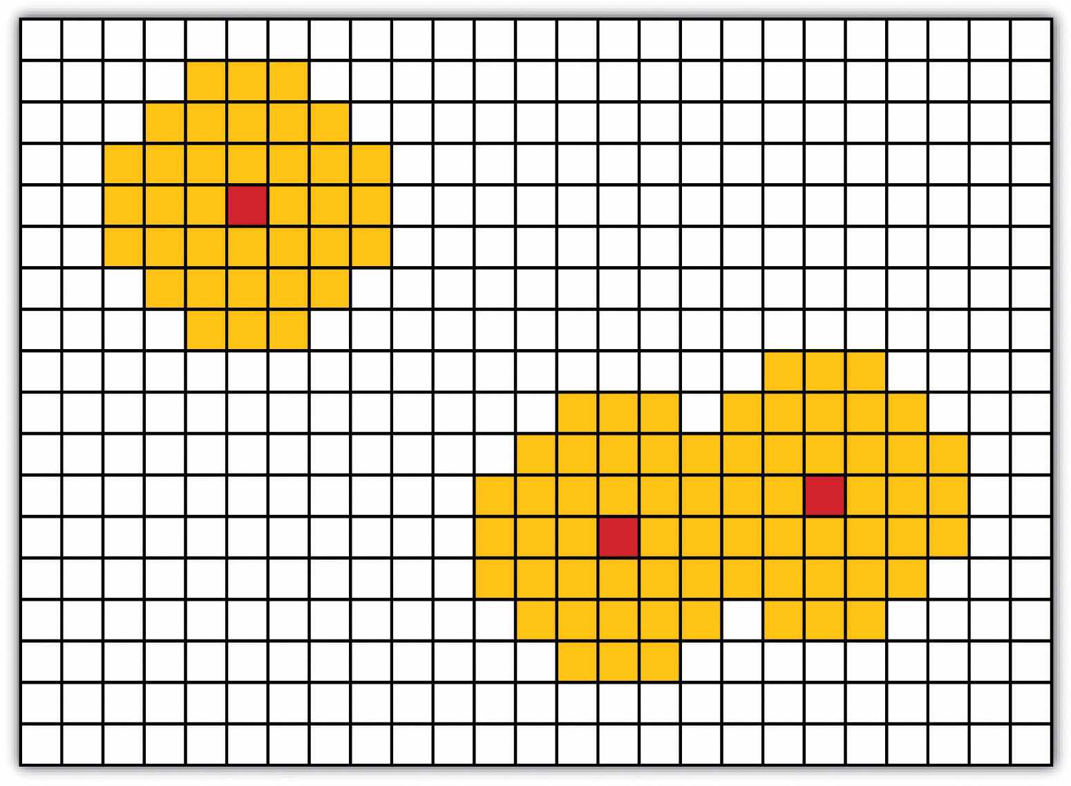
As described in Chapter 7 "Geospatial Analysis I: Vector Operations", buffering is the process of creating an output dataset that contains a zone (or zones) of a specified width around an input feature. In the case of raster datasets, these input features are given as a grid cell or a group of grid cells containing a uniform value (e.g., buffer all cells whose value = 1). Buffers are particularly suited for determining the area of influence around features of interest. Whereas buffering vector data results in a precise area of influence at a specified distance from the target feature, raster buffers tend to be approximations representing those cells that are within the specified distance range of the target (Figure 8.2 "Raster Buffer around a Target Cell(s)"). Most geographic information system (GIS) programs calculate raster buffers by creating a grid of distance values from the center of the target cell(s) to the center of the neighboring cells and then reclassifying those distances such that a “1” represents those cells composing the original target, a “2” represents those cells within the user-defined buffer area, and a “0” represents those cells outside of the target and buffer areas. These cells could also be further classified to represent multiple ring buffers by including values of “3,” “4,” “5,” and so forth, to represent concentric distances around the target cell(s).
Figure 8.2 Raster Buffer around a Target Cell(s)

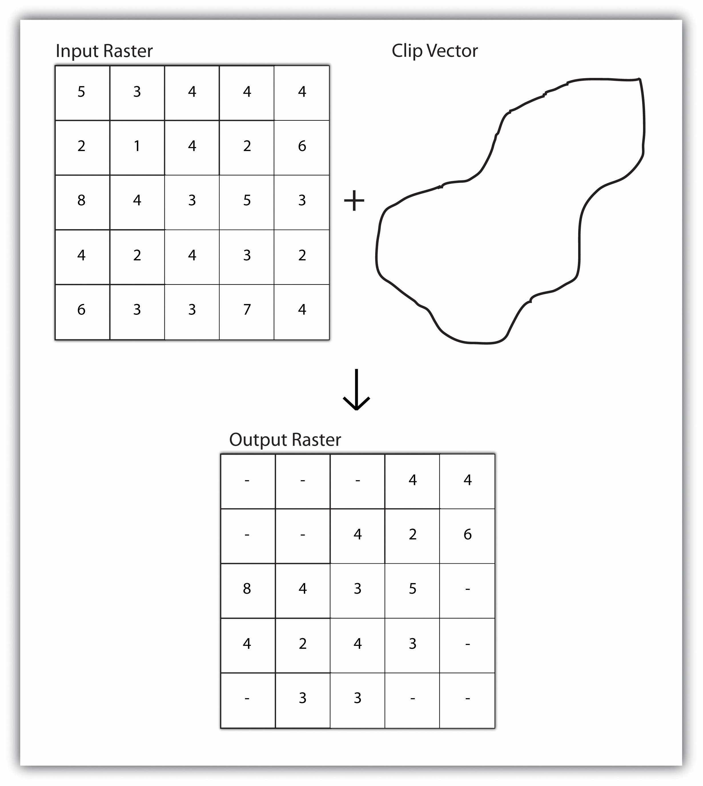
A raster dataset can also be clipped similar to a vector dataset (Figure 8.3 "Clipping a Raster to a Vector Polygon Layer"). Here, the input raster is overlain by a vector polygon clip layer. The raster clip process results in a single raster that is identical to the input raster but shares the extent of the polygon clip layer.
Figure 8.3 Clipping a Raster to a Vector Polygon Layer

Raster overlays are relatively simple compared to their vector counterparts and require much less computational power (Burroughs 1983).Burroughs, P. 1983. Geographical Information Systems for Natural Resources Assessment. New York: Oxford University Press. Despite their simplicity, it is important to ensure that all overlain rasters are coregistered (i.e., spatially aligned), cover identical areas, and maintain equal resolution (i.e., cell size). If these assumptions are violated, the analysis will either fail or the resulting output layer will be flawed. With this in mind, there are several different methodologies for performing a raster overlay (Chrisman 2002).Chrisman, N. 2002. Exploring Geographic Information Systems. 2nd ed. New York: John Wiley and Sons.
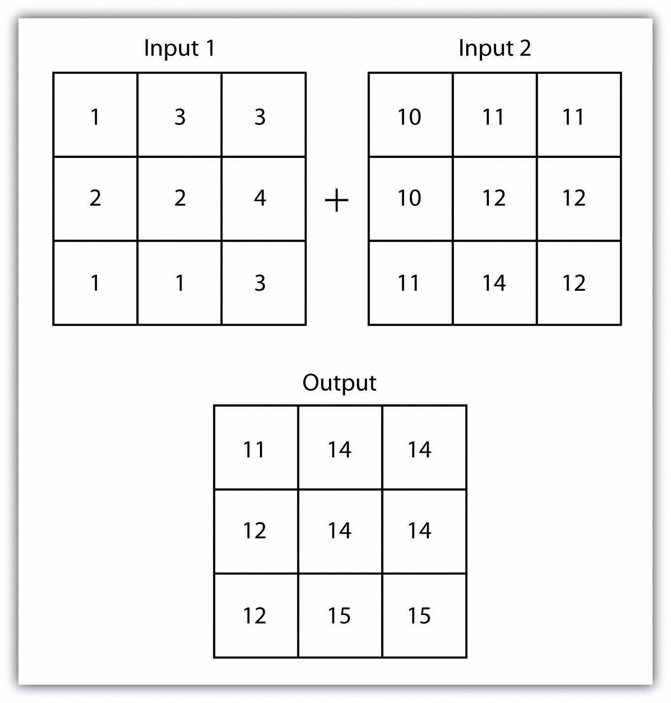
The mathematical raster overlayPixel or grid cell values in each map are combined using mathematical operators to produce a new value in the composite map. is the most common overlay method. The numbers within the aligned cells of the input grids can undergo any user-specified mathematical transformation. Following the calculation, an output raster is produced that contains a new value for each cell (Figure 8.4 "Mathematical Raster Overlay"). As you can imagine, there are many uses for such functionality. In particular, raster overlay is often used in risk assessment studies where various layers are combined to produce an outcome map showing areas of high risk/reward.
Figure 8.4 Mathematical Raster Overlay

Two input raster layers are overlain to produce an output raster with summed cell values.
The Boolean raster overlayPixel or grid cell values in each map are combined using boolean operators to produce a new value in the composite map. method represents a second powerful technique. As discussed in Chapter 6 "Data Characteristics and Visualization", the Boolean connectors AND, OR, and XOR can be employed to combine the information of two overlying input raster datasets into a single output raster. Similarly, the relational raster overlayPixel or grid cell values in each map are combined using relational operators to produce a new value in the composite map. method utilizes relational operators (<, <=, =, <>, >, and =>) to evaluate conditions of the input raster datasets. In both the Boolean and relational overlay methods, cells that meet the evaluation criteria are typically coded in the output raster layer with a 1, while those evaluated as false receive a value of 0.
The simplicity of this methodology, however, can also lead to easily overlooked errors in interpretation if the overlay is not designed properly. Assume that a natural resource manager has two input raster datasets she plans to overlay; one showing the location of trees (“0” = no tree; “1” = tree) and one showing the location of urban areas (“0” = not urban; “1” = urban). If she hopes to find the location of trees in urban areas, a simple mathematical sum of these datasets will yield a “2” in all pixels containing a tree in an urban area. Similarly, if she hopes to find the location of all treeless (or “non-tree,” nonurban areas, she can examine the summed output raster for all “0” entries. Finally, if she hopes to locate urban, treeless areas, she will look for all cells containing a “1.” Unfortunately, the cell value “1” also is coded into each pixel for nonurban, tree cells. Indeed, the choice of input pixel values and overlay equation in this example will yield confounding results due to the poorly devised overlay scheme.