Mean of All Sample Means (μ x)

Statistical analyses are, very often, concerned with the difference between means. A typical example is an experiment designed to compare the mean of a control group with the mean of an experimental group. Inferential statistics used in the analysis of this type of experiment depend on the sampling distribution of the difference between means.

The sampling distribution of the difference between means can be thought of as the distribution that would result if we repeated the following three steps over and over again:

1. Sample n₁ scores from Population 1 and n₂ scores from Population 2;
2. Compute the means of the two samples ( M₁ and M₂);
3. Compute the difference between means M₁−M₂. The distribution of the differences between means is the sampling distribution of the difference between means.

The mean of the sampling distribution of the mean is:

μ_M1−M2 = μ₁−_2,

which says that the mean of the distribution of differences between sample means is equal to the difference between population means. For example, say that mean test score of all 12-year olds in a population is 34 and the mean of 10-year olds is 25. If numerous samples were taken from each age group and the mean difference computed each time, the mean of these numerous differences between sample means would be 34 - 25 = 9.

The variance sum law states that the variance of the sampling distribution of the difference between means is equal to the variance of the sampling distribution of the mean for Population 1 plus the variance of the sampling distribution of the mean for Population 2. The formula for the variance of the sampling distribution of the difference between means is as follows:

${ { \sigma }_{ { M }_{ 1 }-{ M } }^{ 2 } }_{ 2 }=\frac { { \sigma }_{ { M }_{ 1 } }^{ 2 } }{ { n }_{ 1 } } +\frac { { \sigma }_{ { M }_{ 2 } }^{ 2 } }{ { n }_{ 2 } }$.

Recall that the standard error of a sampling distribution is the standard deviation of the sampling distribution, which is the square root of the above variance.

Let's look at an application of this formula to build a sampling distribution of the difference between means. Assume there are two species of green beings on Mars. The mean height of Species 1 is 32, while the mean height of Species 2 is 22. The variances of the two species are 60 and 70, respectively, and the heights of both species are normally distributed. You randomly sample 10 members of Species 1 and 14 members of Species 2.

The difference between means comes out to be 10, and the standard error comes out to be 3.317.

μ_M1−M2 = 32 - 22 = 10

Standard error equals the square root of (60 / 10) + (70 / 14) = 3.317.

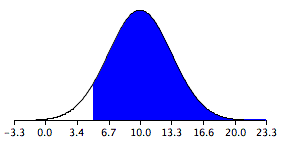
The resulting sampling distribution as diagramed in , is normally distributed with a mean of 10 and a standard deviation of 3.317.

Sampling Distribution of the Difference Between Means

The distribution is normally distributed with a mean of 10 and a standard deviation of 3.317.