In the previous section, we created a sampling distribution out of a population consisting of three pool balls. This distribution was discrete, since there were a finite number of possible observations. Now we will consider sampling distributions when the population distribution is continuous.
What if we had a thousand pool balls with numbers ranging from 0.001 to 1.000 in equal steps? Note that although this distribution is not really continuous, it is close enough to be considered continuous for practical purposes. As before, we are interested in the distribution of the means we would get if we sampled two balls and computed the mean of these two. In the previous example, we started by computing the mean for each of the nine possible outcomes. This would get a bit tedious for our current example since there are 1,000,000 possible outcomes (1,000 for the first ball multiplied by 1,000 for the second.) Therefore, it is more convenient to use our second conceptualization of sampling distributions, which conceives of sampling distributions in terms of relative frequency distributions-- specifically, the relative frequency distribution that would occur if samples of two balls were repeatedly taken and the mean of each sample computed.
Probability Density Function
When we have a truly continuous distribution, it is not only impractical but actually impossible to enumerate all possible outcomes. Moreover, in continuous distributions, the probability of obtaining any single value is zero. Therefore, these values are called probability densities rather than probabilities.
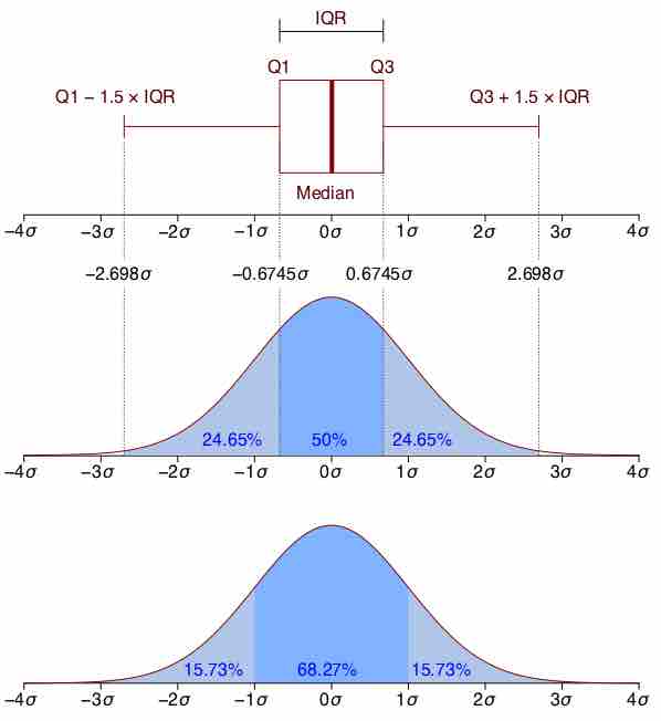
A probability density function, or density of a continuous random variable, is a function that describes the relative likelihood for this random variable to take on a given value. The probability for the random variable to fall within a particular region is given by the integral of this variable's density over the region .

Probability Density Function
Boxplot and probability density function of a normal distribution