In statistical practice, it is possible to miss a real effect simply by not taking enough data. In most cases, this is a problem. For instance, we might miss a viable medicine or fail to notice an important side-effect. How do we know how much data to collect? Statisticians provide the answer in the form of statistical power.
Background
Statistical tests use data from samples to assess, or make inferences about, a statistical population. In the concrete setting of a two-sample comparison, the goal is to assess whether the mean values of some attribute obtained for individuals in two sub-populations differ. For example, to test the null hypothesis that the mean scores of men and women on a test do not differ, samples of men and women are drawn. The test is administered to them, and the mean score of one group is compared to that of the other group using a statistical test such as the two-sample z-test. The power of the test is the probability that the test will find a statistically significant difference between men and women, as a function of the size of the true difference between those two populations. Note that power is the probability of finding a difference that does exist, as opposed to the likelihood of declaring a difference that does not exist (which is known as a Type I error or "false positive").
Factors Influencing Power
Statistical power may depend on a number of factors. Some of these factors may be particular to a specific testing situation, but at a minimum, power nearly always depends on the following three factors:
- The Statistical Significance Criterion Used in the Test: A significance criterion is a statement of how unlikely a positive result must be, if the null hypothesis of no effect is true, for the null hypothesis to be rejected. The most commonly used criteria are probabilities of 0.05 (5%, 1 in 20), 0.01 (1%, 1 in 100), and 0.001 (0.1%, 1 in 1000). One easy way to increase the power of a test is to carry out a less conservative test by using a larger significance criterion, for example 0.10 instead of 0.05. This increases the chance of rejecting the null hypothesis when the null hypothesis is false, but it also increases the risk of obtaining a statistically significant result (i.e. rejecting the null hypothesis) when the null hypothesis is not false.
- The Magnitude of the Effect of Interest in the Population: The magnitude of the effect of interest in the population can be quantified in terms of an effect size, where there is greater power to detect larger effects. An effect size can be a direct estimate of the quantity of interest, or it can be a standardized measure that also accounts for the variability in the population. If constructed appropriately, a standardized effect size, along with the sample size, will completely determine the power. An unstandardized (direct) effect size will rarely be sufficient to determine the power, as it does not contain information about the variability in the measurements.
- The Sample Size Used to Detect the Effect: The sample size determines the amount of sampling error inherent in a test result. Other things being equal, effects are harder to detect in smaller samples. Increasing sample size is often the easiest way to boost the statistical power of a test.
A Simple Example
Suppose a gambler is convinced that an opponent has an unfair coin. Rather than getting heads half the time and tails half the time, the proportion is different, and the opponent is using this to cheat at incredibly boring coin-flipping games. How do we prove it?
Let's say we look for a significance criterion of 0.05. That is, if we count up the number of heads after 10 or 100 trials and find a deviation from what we'd expect – half heads, half tails – the coin would be unfair if there's only a 5% chance of getting a deviation that size or larger with a fair coin. What happens if we flip a coin 10 times and apply these criteria?

Power Curve 1
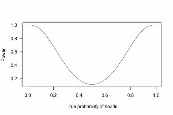
This graph shows the true probability of heads when flipping a coin 10 times.
This is called a power curve. Along the horizontal axis, we have the different possibilities for the coin's true probability of getting heads, corresponding to different levels of unfairness. On the vertical axis is the probability that I will conclude the coin is rigged after 10 tosses, based on the probability of the result.
This graph shows that the coin is rigged to give heads 60% of the time. However, if we flip the coin only 10 times, we only have a 20% chance of concluding that it's rigged. There's too little data to separate rigging from random variation. However, what if we flip the coin 100 times?

Power Curve 2
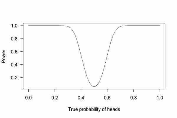
This graph shows the true probability of heads when flipping a coin 100 times.
Or 1,000 times?

Power Curve 3
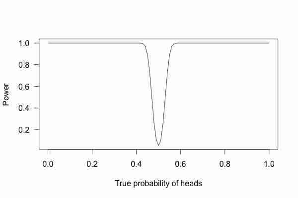
This graph shows the true probability of heads when flipping a coin 1,000 times.
With 1,000 flips, we can easily tell if the coin is rigged to give heads 60% of the time. It is overwhelmingly unlikely that we could flip a fair coin 1,000 times and get more than 600 heads.