
Errors and residuals in statistics
From Wikipedia, the free encyclopedia
In statistics and optimization, the concepts of error and residual are easily confused with each other.
Error is a misnomer; an error is the amount by which an observation differs from its expected value; the latter being based on the whole population from which the statistical unit was chosen randomly. The expected value, being the average of the entire population, is typically unobservable. If the average height in a population of 21-year-old men is 5 feet 9 inches, and one randomly chosen man is 5 feet 11 inches tall, then the "error" is 2 inches; if the randomly chosen man is 5 feet 7 inches tall, then the "error" is −2 inches. The nomenclature arose from random measurement errors in astronomy. It is as if the measurement of the man's height were an attempt to measure the population average, so that any difference between the man's height and the average would be a measurement error.
A residual, on the other hand, is an observable estimate of the unobservable error. The simplest case involves a random sample of n men whose heights are measured. The sample average is used as an estimate of the population average. Then we have:
- The difference between the height of each man in the sample and the unobservable population average is an error, and
- The difference between the height of each man in the sample and the observable sample average is a residual.
- Residuals are observable; errors are not.
Note that the sum of the residuals within a random sample is necessarily zero, and thus the residuals are necessarily not independent. The sum of the errors need not be zero; the errors are independent random variables if the individuals are chosen from the population independently.
- Errors are often independent of each other; residuals are not independent of each other (at least in the simple situation described above, and in many others).
Contents
|
[edit] Example with some mathematical theory
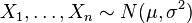
If we assume a normally distributed population with mean μ and standard deviation σ, and choose individuals independently, then we have
and the sample mean
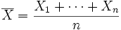
is a random variable distributed thus:

The errors are then

whereas the residuals are
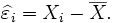
(As is often done, the "hat" over the letter ε indicates an observable estimate of an unobservable quantity called ε.)
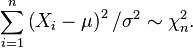
The sum of squares of the errors, divided by σ2, has a chi-square distribution with n degrees of freedom:
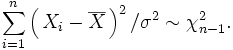
This quantity, however, is not observable. The sum of squares of the residuals, on the other hand, is observable. The quotient of that sum by σ2 has a chi-square distribution with only n − 1 degrees of freedom:
It is remarkable that the sum of squares of the residuals and the sample mean can be shown to be independent of each other. That fact and the normal and chi-square distributions given above form the basis of confidence interval calculations relying on Student's t-distribution. In those calculations one encounters the quotient

in which the σ appears in both the numerator and the denominator and cancels. That is fortunate because in practice one would not know the value of σ2.