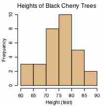
A histogram is a graphical representation of the distribution of data. More specifically, a histogram is a representation of tabulated frequencies, shown as adjacent rectangles, erected over discrete intervals (bins), with an area equal to the frequency of the observations in the interval. First introduced by Karl Pearson, it is an estimate of the probability distribution of a continuous variable.

A histogram has both a horizontal axis and a vertical axis. The horizontal axis is labeled with what the data represents (for instance, distance from your home to school). The vertical axis is labeled either frequency or relative frequency. The graph will have the same shape with either label. An advantage of a histogram is that it can readily display large data sets (a rule of thumb is to use a histogram when the data set consists of 100 values or more). The histogram can also give you the shape, the center, and the spread of the data.

The categories of a histogram are usually specified as consecutive, non-overlapping intervals of a variable. The categories (intervals) must be adjacent and often are chosen to be of the same size. The rectangles of a histogram are drawn so that they touch each other to indicate that the original variable is continuous.

Frequency and Probability Distributions

In statistical terms, the frequency of an event is the number of times the event occurred in an experiment or study. The relative frequency (or empirical probability) of an event refers to the absolute frequency normalized by the total number of events:

$\displaystyle f_i=\frac{n_i}{N} = \frac{n_i}{\sum_i n_i}$

Put more simply, the relative frequency is equal to the frequency for an observed value of the data divided by the total number of data values in the sample.

The height of a rectangle in a histogram is equal to the frequency density of the interval, i.e., the frequency divided by the width of the interval. A histogram may also be normalized displaying relative frequencies. It then shows the proportion of cases that fall into each of several categories, with the total area equaling one.

As mentioned, a histogram is an estimate of the probability distribution of a continuous variable. To define probability distributions for the simplest cases, one needs to distinguish between discrete and continuous random variables. In the discrete case, one can easily assign a probability to each possible value. For example, when throwing a die, each of the six values 1 to 6 has the probability 1/6. In contrast, when a random variable takes values from a continuum, probabilities are nonzero only if they refer to finite intervals. For example, in quality control one might demand that the probability of a "500 g" package containing between 490 g and 510 g should be no less than 98%.

Intuitively, a continuous random variable is the one which can take a continuous range of values — as opposed to a discrete distribution, where the set of possible values for the random variable is, at most, countable. If the distribution of $x$ is continuous, then $x$ is called a continuous random variable and, therefore, has a continuous probability distribution. There are many examples of continuous probability distributions: normal, uniform, chi-squared, and others.

The Histogram

This is an example of a histogram, depicting graphically the distribution of heights for 31 Black Cherry trees.