The number of independent ways by which a dynamical system can move without violating any constraint imposed on it is known as "degree of freedom. " The degree of freedom can be defined as the minimum number of independent coordinates that completely specify the position of the system.
Consider this example: To compute the variance, first sum the square deviations from the mean. The mean is a parameter, a characteristic of the variable under examination as a whole, and a part of describing the overall distribution of values. Knowing all the parameters, you can accurately describe the data. The more known (fixed) parameters you know, the fewer samples fit this model of the data. If you know only the mean, there will be many possible sets of data that are consistent with this model. However, if you know the mean and the standard deviation, fewer possible sets of data fit this model.
In computing the variance, first calculate the mean, then you can vary any of the scores in the data except one. This one score left unexamined can always be calculated accurately from the rest of the data and the mean itself.
As an example, take the ages of a class of students and find the mean. With a fixed mean, how many of the other scores (there are N of them remember) could still vary? The answer is N-1 independent pieces of information (degrees of freedom) that could vary while the mean is known. One piece of information cannot vary because its value is fully determined by the parameter (in this case the mean) and the other scores. Each parameter that is fixed during our computations constitutes the loss of a degree of freedom.
Imagine starting with a small number of data points and then fixing a relatively large number of parameters as we compute some statistic. We see that as more degrees of freedom are lost, fewer and fewer different situations are accounted for by our model since fewer and fewer pieces of information could, in principle, be different from what is actually observed.
Put informally, the "interest" in our data is determined by the degrees of freedom. If there is nothing that can vary once our parameter is fixed (because we have so very few data points, maybe just one) then there is nothing to investigate. Degrees of freedom can be seen as linking sample size to explanatory power.
The degrees of freedom are also commonly associated with the squared lengths (or "sum of squares" of the coordinates) of random vectors and the parameters of chi-squared and other distributions that arise in associated statistical testing problems.
Notation and Residuals
In equations, the typical symbol for degrees of freedom is
In fitting statistical models to data, the random vectors of residuals are constrained to lie in a space of smaller dimension than the number of components in the vector. That smaller dimension is the number of degrees of freedom for error. In statistical terms, a random vector is a list of mathematical variables each of whose value is unknown, either because the value has not yet occurred or because there is imperfect knowledge of its value. The individual variables in a random vector are grouped together because there may be correlations among them. Often they represent different properties of an individual statistical unit (e.g., a particular person, event, etc.).
A residual is an observable estimate of the unobservable statistical error. Consider an example with men's heights and suppose we have a random sample of n people. The sample mean could serve as a good estimator of the population mean. The difference between the height of each man in the sample and the observable sample mean is a residual. Note that the sum of the residuals within a random sample is necessarily zero, and thus the residuals are necessarily not independent.
Perhaps the simplest example is this. Suppose X1,...,Xn are random variables each with expected value μ, and let
be the "sample mean. " Then the quantities
are residuals that may be considered estimates of the errors Xi − μ. The sum of the residuals is necessarily 0. If one knows the values of any n − 1 of the residuals, one can thus find the last one. That means they are constrained to lie in a space of dimension n − 1, and we say that "there are n − 1 degrees of freedom for error. "

Degrees of Freedom
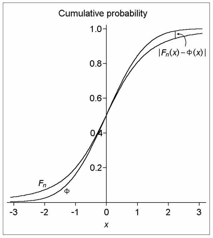
This image illustrates the difference (or distance) between the cumulative distribution functions of the standard normal distribution (Φ) and a hypothetical distribution of a standardized sample mean (Fn). Specifically, the plotted hypothetical distribution is a t distribution with 3 degrees of freedom.