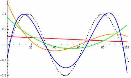
For a set of data containing two (or more) quantitative properties, statisticians use functions to denote a relationship between two or more distinct properties. When we find a function that lies reasonably close to the collected data points, we create a trend line which says how one property behaves as a function of the other ones. We call this curve fitting. Then we can use this to make predictions about the former property once we know something about the others.
For example, if you measure the height of
Polynomial and rational functions are easy to work with because you only need to make use of elementary operations.
Recall that a polynomial function has the following form:
where
Polynomial functions are very simple in form and easy to use, but they have limitations with regard to statistical modeling. They can take on only a limited number of shapes and are particularly ill-suited to modeling asymptotes. They are finite when
This need not be a problem. For lots of datasets, their are no asymptotes and data is more or less bounded. (For example, there are no humans who are
Polynomials have also lots of advantages:
- They are well studied: a lot of their properties are known.
- They are easy to compute, using only multiplication and addition.
- They are closed under rescaling or changing of locations: if we change a kilometer to a mile we still get a polynomial.
To deal with the asymptotic problems of polynomials, we also use rational functions:
A rational function is the ratio of two polynomial functions and has the following form:
Here, n and m define the degrees of the numerator and denominator, respectively, and together, they define the degree of the polynomial. For example, if
Rational functions are a little more complex in form than polynomial functions, but they have an advantage in that they can take on a much greater range of shapes and can effectively model asymptotes. They are also more accurate than polynomial functions both inside and outside the limits of collected data. However, rational functions sometimes include undesirable asymptotes that can disrupt an otherwise smooth trend line. They are also a little bit more difficult to compute, since you also need division to compute them. However, they still run fast.

Curve fitting
Polynomial curves generated to fit points (black dots) of a sine function: The red line is a first degree polynomial; the green is a second degree; the orange is a third degree; and the blue is a fourth degree.
Polynomials and rational functions are used for approximation in many everyday devices. For example, every time we take a picture with a smartphone, our phone looks at some data points and fills in the appropriate colors in the blanks, thus saving us a lot of memory, with the help of rational functions. Every time we say something through the phone, our phone tries to reduce the background noise by approximating our sound for short periods of time, again with the help of rational functions.