Google Sheets
Sorting and Filtering Data
Introduction
Google Sheets allows you to analyze and work with a significant amount of data. As you add more content to your spreadsheet, organizing information in it becomes important. Google Sheets allows you reorganize your data by sorting and applying filters to it. You can sort your data by arranging it alphabetically or numerically, or you can apply a filter to narrow down the data and hide some of it from view.
In this lesson, you will learn how to sort data to better view and organize the contents of your spreadsheet. You will also learn how to filter data to display only the information you need.
Types of sorting
When sorting data, it's important to first decide if you want the sort to apply to the entire sheet or to a selection of cells.
-
Sort sheet
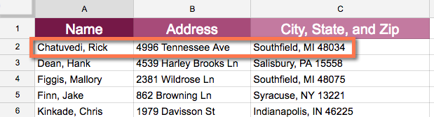
organizes all of the data in your spreadsheet by one column. Related information across each row is kept together when the sort is applied. In the image below, the Name column has been sorted to display client names in alphabetical order. Each client's address information has been kept with each corresponding name.
-
Sort range
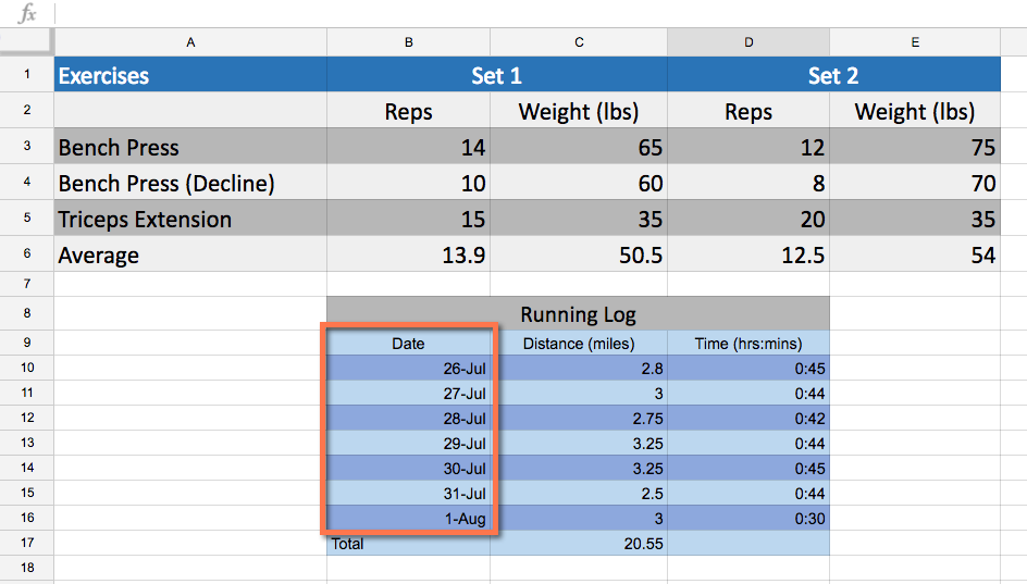
sorts the data in a range of cells, which can be helpful when working with a sheet that contains several tables. Sorting a range will not affect other content on the worksheet.
To sort a sheet:
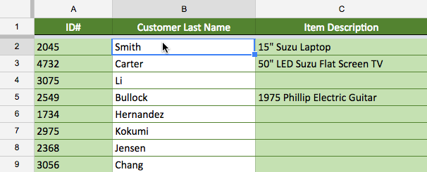
In our example, we'll sort a list of customers alphabetically by last name . In order for sorting to work correctly, your worksheet should include a header row , which is used to identify the name of each column. We will freeze the header row so the header labels will not be included in the sort.
-
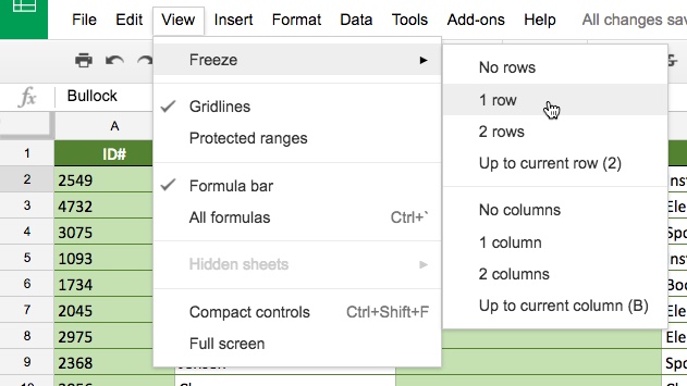
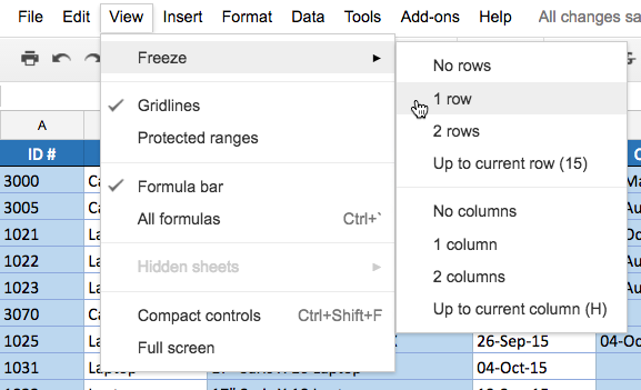
Click
View
and hover the mouse over
Freeze
. Select
1 row
from the menu that appears.
-
The header row freezes. Decide which
column
will be sorted, then click a
cell
in the column.
-
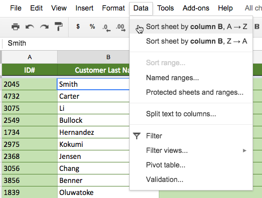
Click
Data
and select
Sort Sheet by column, A-Z
(ascending) or
Sort Sheet by column, Z
-
A
(descending). In our example, we'll select Sort Sheet by column, A-Z.
-
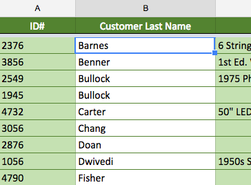
The sheet will be sorted according to your selection.
To sort a range:
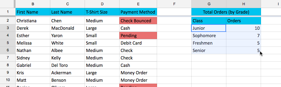
In our example, we'll select a secondary table in a T-shirt order form to sort the number of shirts that were ordered by class.
-
Select the
cell range
you want to sort. In our example, we'll select cell range
G3:H6
.
-
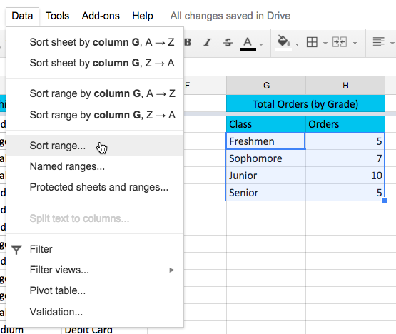
Click
Data
and select
Sort range
from the drop-down menu.
-
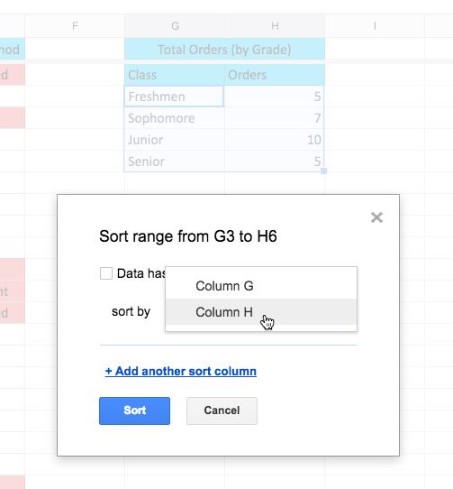
The Sorting dialog box appears. Select the desired
column
you want to sort by.
-
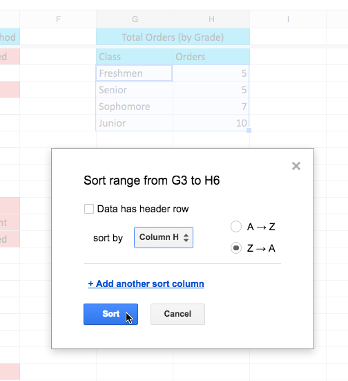
Select
ascending
or
descending
. In our example, we'll select descending (Z-A). Then click
Sort
.
-
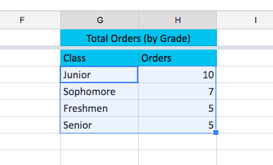
The range will be sorted according to your selections (in our example, the data has been sorted in descending order according to the Orders column).
To create a filter:
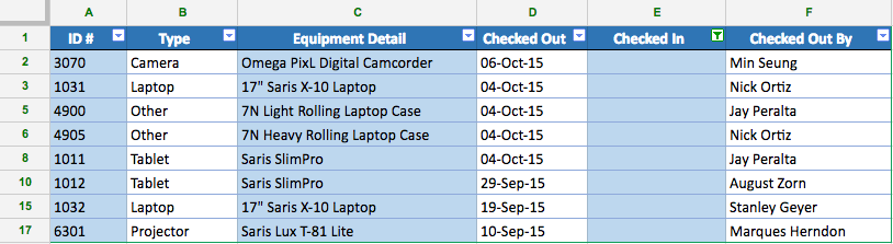
In our example, we'll apply a filter to an equipment log worksheet to display only the laptops and projectors that are available for checkout. In order for sorting to work correctly, your worksheet should include a header row , which is used to identify the name of each column. We will freeze the header row so the header labels will not be included in the filter.
-
Click
View
and hover the mouse over
Freeze
. Select
1 row
from the menu that appears.
-
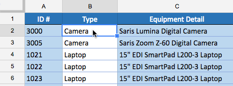
Click any
cell
that contains data.
-
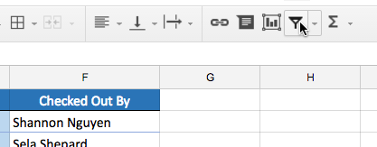
Click the Filter button.

-
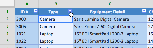
A drop-down arrow appears in each column header.
-
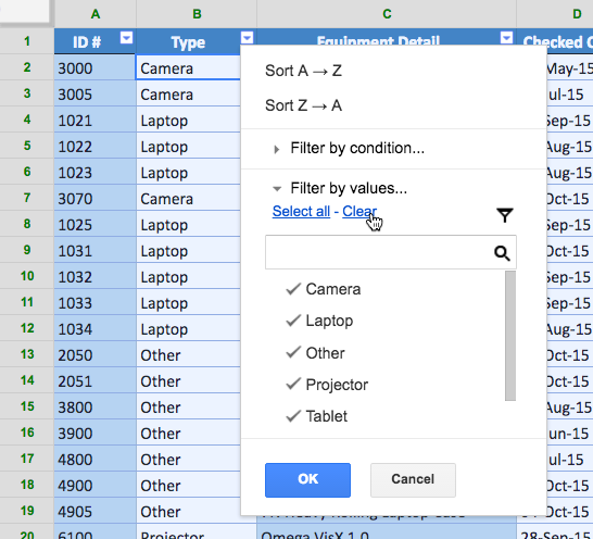
Click the
drop-down arrow
for the column you want to filter. In our example, we will filter column
B
to view only certain types of equipment.
-
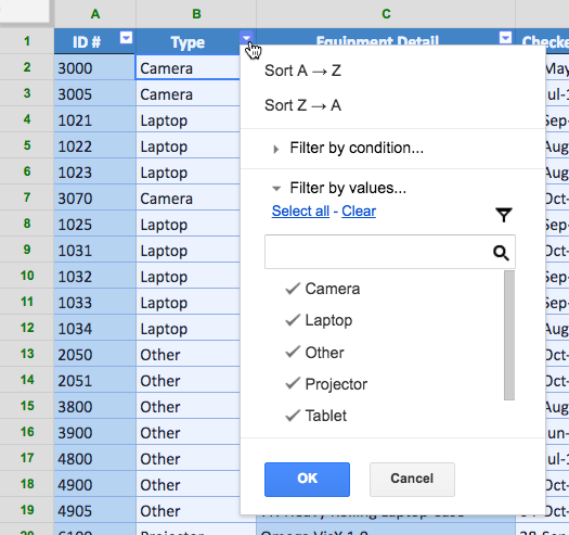
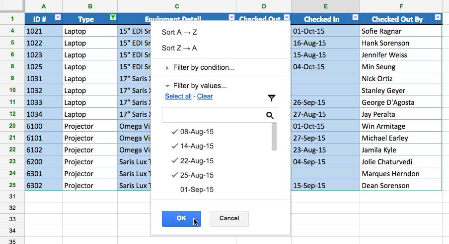
Click
Clear
to remove all of the checks.
-
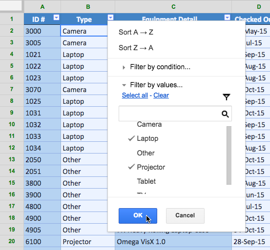
Select the data you want to filter, then click
OK
. In this example, we will check
Laptop
and
Projector
to view only these types of equipment.
-
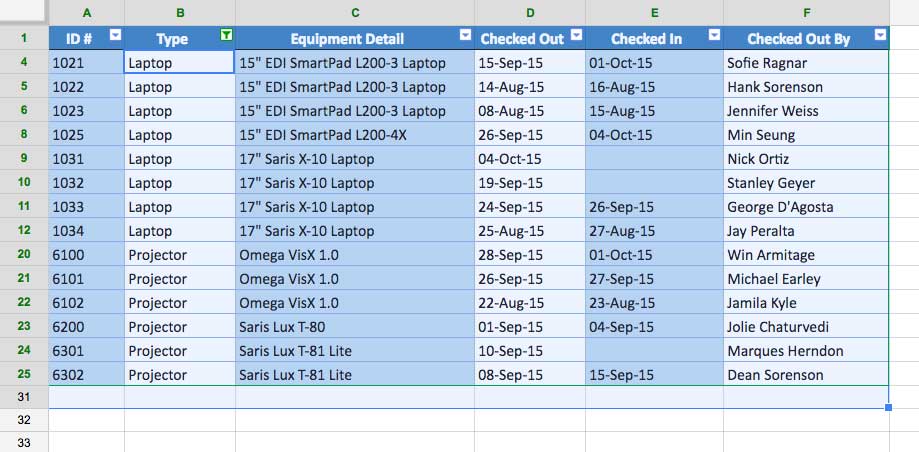
The data will be
filtered
, temporarily hiding any content that doesn't match the criteria. In our example, only laptops and projectors are visible.
Applying multiple filters
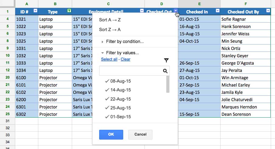
Filters are cumulative , which means you can apply multiple filters to help narrow down your results. In this example, we've already filtered our worksheet to show laptops and projectors, and we'd like to narrow it down further to only show laptops and projectors that were checked out in August.
-
Click the
drop-down arrow
for the column you want to filter. In this example, we will add a filter to column
D
to view information by date.
-
Check
or
uncheck
the boxes depending on the data you want to filter, then click
OK
. In our example, we'll uncheck everything except for
August
.
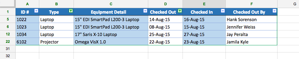
-
The new filter will be applied. In our example, the worksheet is now filtered to show only laptops and projectors that were checked out in August.
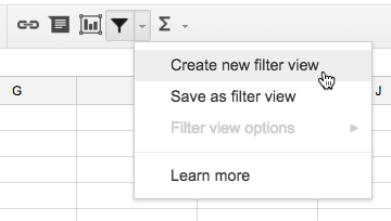
If you're collaborating with others on a sheet, you can create a filter view . Creating a filter view allows you to filter data without affecting other people's view of the data; it only affects your own view. It also allows you to name views and save multiple views. You can create a filter view by clicking the drop-down arrow next to the Filter button.
To clear all filters:
-
Click the
Filter button
, and the spreadsheet will return to its original appearance.
Challenge!
- Open our example file . Make sure you're signed in to Google, then click File > Make a copy .
- Select the Equipment Log tab if it is not already open.
- Freeze row 1.
-
Sort
the spreadsheet by the
Checked Out
date from most recent to the oldest.
Hint: Sort by column D from Z to A. -
S
ort the range
A2:F9 by column
B
from
A to Z
.
Hint: Make sure the box next to data has header row is left unchecked. -
Filter
the spreadsheet so it only shows equipment that has never been checked in.
Hint: Filter column E to show cells that are empty. -
When you're finished, your spreadsheet should look like this: